 AI insights
 About us
 Careers
 Security
 Customer reviews
 Contact us
 Affiliate program
 Solution partners
 Looker Studio templates
 Tableau templates
 Facebook Ads templates
 Google Ads templates
 Data fields & Metrics
 AI prompt library & Guides
 Product documentation
 API documentation
 Case studies
 Blog
Blog Data models
 Windsor vs Supermetrics
 Windsor vs Fivetran
 Windsor vs Portermetrics
 Last updated: 21 May 2025
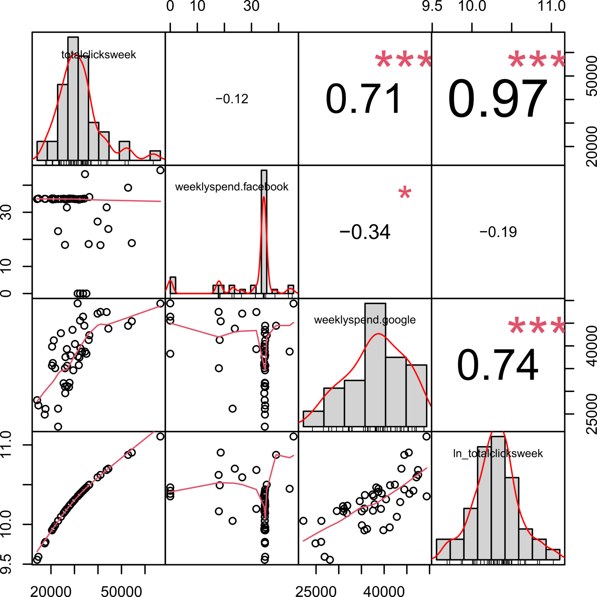

In this guide you will learn how to fetch your marketing data and apply a Marketing Mix Model to elucidate which source presents the best marketing performance. Marketing Mix Modelling is a statistical analyses such as multivariate regressions on sales and marketing time series data to estimate the impact of various marketing tactics on a given variable related to reward (e.g., number of clicks).
Our aim will be to elucidate which marketing platform presents the highest number of clicks per spend for the last year. More concretely, we will consider Facebook and Google Ads data.
First, we will use Windsor.ai API to get our marketing data from Facebook Ads and Google Ads. Then, we will clean the data and prepare it for the analyses. Finally we will perform the analysis to answer our question.
Get started
First of all we need to install the packages we will use.
install.packages(c("facebookadsR", "googleadsR", "dplyr", "ggplot2", "PerformanceAnalytics", "mctest", "lmtest"), dependencies = T)Once we have downloaded the packages, we can load them.
library(facebookadsR) # get Facebook Ads data from windsor.ai API
library(googleadsR) # get Google Ads data from windsor.ai API
library(dplyr) # data cleaning
library(ggplot2) # plotting
library(PerformanceAnalytics) # to calculate correlations
library(mctest) # to evaluate models assumptions (lineality)
library(lmtest) # to evaluate models assumptions (homocedasticity)
Get data using Windsor.ai API
Now we will use two packages that allows us to get marketing data from windsor.ai API for Facebook (facebookadsR) and for Google (googleadsR).All you need before starting to get your data is to create and account in windsor.ai and get an API key. You have a 30 days free trial.
By using the following code, you will download marketing data from 2022-01-01 to now. More concretely, we are interested in the variables clicks, representing the number of clicks which will be our measure related to marketing performance and spend as a measure of the money invested in each platform per date. We will also need a variable identifying the source (here, Facebook or Google) and the date.
Then, we can unify the data into an integrated data base containing both Facebook and Google Ads marketing data.
my_facebook_data <- facebookadsR::fetch_facebookads(api_key = "your api key",
date_from = "2022-01-01",
date_to = Sys.Date(),
fields = c("source", "date", "clicks", "spend")) %>%
dplyr::mutate(source = as.character(source),
date = as.Date(date),
clicks = as.numeric(clicks),
spend = as.numeric(spend)) %>%
aggregate(. ~ date + source, FUN = sum)

my_google_data <- googleadsR::fetch_googleads(api_key = "your api key",
date_from = "2022-01-01",
date_to = Sys.Date(),
fields = c("source", "date", "clicks", "spend")) %>%
dplyr::mutate(source = as.character(source),
date = as.Date(date),
clicks = as.numeric(clicks),
spend = as.numeric(spend)) %>%
aggregate(. ~ date + source, FUN = sum)

my_integrated_data <- rbind(my_facebook_data, my_google_data)
Let’s have a quick look at the data we just downloaded and unified.
glimpse(my_integrated_data)#> Rows: 607
#> Columns: 4
#> $ date <date> 2022-01-01, 2022-01-02, 2022-01-03, 2022-01-04, 2022-01-05, 20…
#> $ source <chr> “facebook”, “facebook”, “facebook”, “facebook”, “facebook”, “fa…
#> $ clicks <dbl> 10, 9, 2, 2, 8, 6, 5, 3, 5, 4, 4, 3, 3, 4, 4, 1, 3, 7, 4, 3, 3,…
#> $ spend <dbl> 4.89, 5.05, 5.01, 4.95, 4.95, 5.02, 5.10, 4.92, 4.86, 4.91, 4.9…
Clean data
Now, we will proceed to prepare our data for the analyses. We will start by aggregating the data by week. First, we need to create a new varaible identifying each week for the period we have.
my_integrated_data$week <- lubridate::week(my_integrated_data$date)Then, we can aggregate the data by week as it follows:
weekly_spend_df <- aggregate(spend ~ week + source,
data = my_integrated_data,
sum) %>%
rename(weeklyspend = spend)

weekly_clicks_df <- aggregate(clicks ~ week,
data = my_integrated_data,
sum) %>%
rename(totalclicksweek = clicks)

weekly_df <- merge(weekly_spend_df,
weekly_clicks_df,
by="week")
Let’s have a look at the data before we further proceed.
head(weekly_df)#> week source weeklyspend totalclicksweek
#> 1 1 facebook 34.97 17345
#> 2 1 google 24877.29 17345
#> 3 2 facebook 34.88 14109
#> 4 2 google 28053.36 14109
#> 5 3 facebook 35.05 14653
#> 6 3 google 26890.79 14653
Let’s have a look at the structure of the data too:
glimpse(weekly_df)#> Rows: 88
#> Columns: 4
#> $ week <dbl> 1, 1, 2, 2, 3, 3, 4, 4, 5, 5, 6, 6, 7, 7, 8, 8, 9, 9, …
#> $ source <chr> “facebook”, “google”, “facebook”, “google”, “facebook”…
#> $ weeklyspend <dbl> 34.97, 24877.29, 34.88, 28053.36, 35.05, 26890.79, 261…
#> $ totalclicksweek <dbl> 17345, 17345, 14109, 14109, 14653, 14653, 17673, 17673…
Finally, in order to apply marketing mix modelling, we will need to transform the data from narrow to wide format.
weekly_reshaped_clicks <- reshape(weekly_df,
idvar = c("totalclicksweek","week"),
timevar = "source",
direction = "wide")

weekly_reshaped_clicks[is.na(weekly_reshaped_clicks)] <- 0
This is how our wide data looks like:
head(weekly_reshaped_clicks)#> week totalclicksweek weeklyspend.facebook weeklyspend.google
#> 1 1 17345 34.97 24877.29
#> 3 2 14109 34.88 28053.36
#> 5 3 14653 35.05 26890.79
#> 7 4 17673 34.94 26123.59
#> 9 5 23039 34.91 22211.05
#> 11 6 26069 34.73 29579.07
Calculate correlations
First of all is always important to see how our variables are related. We can do it by calculating their correlations.
chart.Correlation(weekly_reshaped_clicks[, -1],
histogram = TRUE,
pch=19)
By looking at the variables distribution (diagonal of the plot) we can see how our response variable, number clicks per week presents a rather skewed distribution. We can try to improve that by log-transforming it, which will probably help to meet the normality assumption of linear models.
Marketing Mix Modelling
Now, we are ready to apply our Marketing Mix Model. We will use the lm function, which implements a linear model. We will set the total clicks per week (log-transformed to improve its normality) as the response variable related to reward and weekly spend in Facebook and weekly spend in Google as our predictors of interest. By calling the summary of the model we can further see and interpret our results.
mmm_1 <- lm(ln_totalclicksweek ~ weeklyspend.facebook + weeklyspend.google,
data = weekly_reshaped_clicks)
summary(mmm_1)
#>
#> Call:
#> lm(formula = ln_totalclicksweek ~ weeklyspend.facebook + weeklyspend.google,
#> data = weekly_reshaped_clicks)
#>
#> Residuals:
#> Min 1Q Median 3Q Max
#> -0.4418 -0.1013 0.0423 0.1379 0.3963
#>
#> Coefficients:
#> Estimate Std. Error t value Pr(>|t|)
#> (Intercept) 8.891e+00 2.384e-01 37.288 < 2e-16 ***
#> weeklyspend.facebook 2.130e-03 3.122e-03 0.682 0.499
#> weeklyspend.google 3.490e-05 4.954e-06 7.045 1.11e-08 ***
#> —
#> Signif. codes: 0 ‘***’ 0.001 ‘**’ 0.01 ‘*’ 0.05 ‘.’ 0.1 ‘ ‘ 1
#>
#> Residual standard error: 0.2179 on 43 degrees of freedom
#> Multiple R-squared: 0.552, Adjusted R-squared: 0.5312
#> F-statistic: 26.49 on 2 and 43 DF, p-value: 3.176e-08
So, we can see how there is a significant positive effect of the spend in Google with the number of clicks, meaning that the number of spend in this platform Ads present a statistical relationship with a higher number of clicks. So we can answer our question based on our data, which points that investment in Google Ads is translated into a higher number of clicks. This model can be applied then to multiple platforms to compare them and see which ones are related to different response variables related to reward, providing extremely useful insights that will allow us to elucidate which are the platforms that are performing better.
Model assumptions
Finally, we need to test if model assumptions are meet in order to know if we can trust our results. Specifically, we will test for clolinearity and homocedasticity. To do so we will use two premade functions. If the p-value of the tests are > 0.05, we can confidently say that our model meets the assumptions of linear models.
First, let’s check for colinearity:
imcdiag(mmm_1, method = "VIF")#>
#> Call:
#> imcdiag(mod = mmm_1, method = “VIF”)
#>
#>
#> VIF Multicollinearity Diagnostics
#>
#> VIF detection
#> weeklyspend.facebook 1.1317 0
#> weeklyspend.google 1.1317 0
#>
#> NOTE: VIF Method Failed to detect multicollinearity
#>
#>
#> 0 –> COLLINEARITY is not detected by the test
#>
#> ===================================
No colinearity detected.
Now, let’s check for heterocedasticity:
lmtest::bptest(mmm_1)#>
#> studentized Breusch-Pagan test
#>
#> data: mmm_1
#> BP = 1.3884, df = 2, p-value = 0.4995
No heterocedasticity detected, so linear models assumptions are meet and we can confidently trust our results.

